
December saw the release of the 2020 edition of the Human Freedom Index, published jointly by the Cato Institute and the Fraser Institute. The index is a massive effort that combines an Economic Freedom Index developed by the Fraser Institute with a separate index of personal freedom compiled by Cato. The freedom indexes and the data behind them are a treasure trove for data junkies like me. This commentary takes the data for a test drive by exploring a key finding of the Cato-Fraser report: that economic freedom and personal freedom go hand in hand.
Economic and personal freedom: A first look
The Human Freedom Index comprises 76 individual indicators, divided into 12 groups. Five of the groups cover economic freedom: Size of government; legal system and property rights (LSPR); sound money; freedom of trade; and regulation. The remaining seven groups cover personal freedom, including rule of law; safety and security; freedom of movement; religion; association, assembly, and civil society; expression and information; and identity and relationships.
Figure 4 in the freedom report is a scatter plot that shows a strong correlation between economic and personal freedom. My version of the chart looks like this:
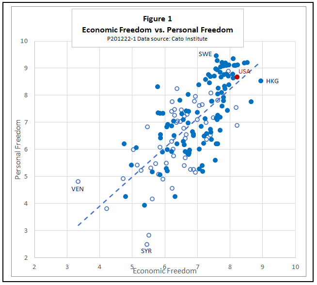
The points in the diagram cluster around a positively sloping trendline, showing that countries with freer economies, by and large, tend also to enjoy greater personal freedom. Statistically, differences in economic freedom account for just over half of the variance in personal freedom.[1] Sweden has the highest personal freedom score, while Hong Kong has the highest economic freedom score.[2]
The analysis section that follows explores what goes on behind the scenes to produce the striking relationship between economic and personal freedom. In a concluding section, I make several suggestions for strengthening the economic freedom portion of the index. Readers who are willing to take my conclusions at face value without examining the statistical details of how I reach them can skip the analysis section and go directly to the conclusions.
Analysis
The Cato Human Freedom Index covers 162 countries in all, but many countries lack data for one or more of the 76 individual indicators in the data set. Group scores for those countries are estimated based on the remaining indicators within each group for which data are available. In my analysis, I will frequently want to dig below the group scores to the individual indicators. For that reason, I will use only the subsample of 107 countries for which there are no missing data. Those countries are shown as solid dots in Figure 1. Countries represented by empty dots are missing data for one or more indicators. The fit between the two types of freedom for the 107-country subsample (R2 = 0.48) is slightly less close than that for the 162 countries as a whole (R2 = 0.51), but the difference is not statistically significant.[3]
The fact that the summary score for economic freedom accounts for half of the cross-country variance in personal freedom can be considered a strong result, especially in the social sciences, which deal with notoriously variable human behavior and hard-to-measure concepts. However, that top-line result by no means exhausts the explanatory power of the available data. We need to dig deeper, exploring the separate economic freedom groups and the individual indicators within them.
As a first step, we can use the five economic freedom groups as separate control variables in a multiple regression, with personal freedom as the response variable. When we do so, the share of the cross-country variance in personal freedom jointly explained by economic freedom rises from just half to nearly three-quarters (R2 = 0.74). The regression results show that the five economic freedom groups are not all of equal importance. Each of the group scores except regulation has at least a marginally significant effect on personal freedom, but nearly all of the effect comes from two groups, legal systems and property rights (LSPR) and international trade. The regression coefficient for sound money is negative; that is, personal freedom tends to be higher in countries where the score for the sound money group is lower.[4] (An Online Supplement to this report gives complete results for these and other statistical tests and regressions. See sheet OS1 for the results cited in this paragraph.)
The above results further vindicate the notion that economic freedom and personal freedom are strongly related, but there is more to learn. The next step is to examine the individual indicators within each economic freedom group to see which of them contribute most to the relationship, and how.
Size of government. The first group, which measures the size of government, comprises five indicators: government consumption expenditures, transfer payments, top marginal tax rates, government investment, and government ownership of assets. We can begin by applying some standard tests to see whether these indicators form a coherent group – colloquially speaking, whether they are all “apples” or whether they mix “apples” and “oranges.”
One such test is called Cronbach’s alpha, a statistic ranging from 0 to 1 that measures how closely related items in a set of indicators are to one another. A typical application of Cronbach’s alpha might be to evaluate a set of questions designed to predict whether a job applicant would do well in a sales position. If adding a new item to the questionnaire increases the value of alpha, that item is likely to improve predictions. If adding a question reduces alpha, the questionnaire is likely to be more useful without it. There is no magic value of Cronbach’s alpha that makes a set of indicators reliable, but as a rule of thumb, a value of 0.70 or better can be considered encouraging. Very high values of alpha, 0.90 or above, may indicate that there is redundancy among the items. For example, an alpha of 0.95 for the sales questionnaire might mean that a version with fewer questions could predict job performance just as well.
Principal component analysis is another technique that is useful in the search for patterns in large data sets. If the variables in a data set are closely related, a single principal component, or a small number of such components, can be used in place of the complete set with little loss of information. If the items in the original data set are not closely related to one another, they cannot usefully be reduced to one or a few principal components.
In the case of the “size of government” group, Cronbach’s alpha is very low (α = 0.25), raising a red flag as to its statistical coherence. The first principal component accounts for about half of the variation in the data within this group and the second principal component about 25 percent. Government consumption, transfers, and tax rates affect the components differently from government investment and ownership, suggesting, figuratively, that the first three are “apples” while the last two are “oranges.”
It is important to point out that Cronbach’s alpha does not measure the quality or usefulness of the individual indicators, but only the extent to which they form a statistically coherent group. If they do form such a group, then a summary score for the group, such as a simple average or weighted average, will be useful for analytical purposes. If the items in the group are unrelated, an average score is not likely to tell us much, even if we could learn a great deal from some of the individual elements in the group. In this case, the “size of government” group does not appear to be tightly consistent, suggesting that using the group score in place of the individual variables carries a risk of degrading the explanatory power of the data.
Multiple regression analysis confirms that impression. A regression using the five individual indicators from the size of government group along with the summary scores for the other four groups as control variables produces a multiple R2 of 0.82, a significant increase from the R2 of 0.74 when only the group scores were used.
Of the five components of size of government, only state ownership of assets has a significant positive association with personal freedom. In fact, state ownership alone has more explanatory power than the size of government group score. Accordingly, I will use it in place of the group score for size of government in further regressions discussed below.
Before leaving the size of government group, it is worth looking briefly at the signs of the coefficients obtained in the above regressions. In the regression using only the five group scores as controls, the coefficient for the size of government group is positive and marginally significant. Keep in mind that the score is constructed so that a higher value means a smaller government, so the positive coefficient for the group score is consistent with the libertarian a priori that larger government means less freedom.
In regressions using the five individual components of size of government separately, most of the coefficients are not significantly different from zero. Even so, the sign of a statistically insignificant coefficient still carries some information. A positive sign means that the relationship of that control variable with the response variable is at least somewhat more likely to be positive than negative, and vice versa. It is noteworthy, then, that the signs for the three fiscal indicators (government consumption, transfer payments, and top marginal tax rate) are all negative. That suggests that the libertarian a priori is more likely to be false than true for fiscal measures of the size of government, even though indicators of government ownership are positively related to personal freedom. (See OS2 for details of these statistical findings regarding size of government.)
Legal system and property rights. The LSPR group includes eight indicators, measuring judicial independence, impartiality of courts, protection of property rights, integrity of the legal system, contract enforcement, reliability of police, and regulatory costs of property sales. In contrast to the “size of government” group, the LSPR group has a high degree of statistical reliability. Cronbach’s alpha is a strong 0.93. That increases slightly, to 0.96, if the last two indicators (police and property sales) are dropped. Evidently, there is some redundancy in this group. Multiple regression analysis does not find any one component of LSPR to stand out from the others.
Some readers will recognize that the first six indicators in the Cato/Fraser LSPR group closely parallel a variable that I have called “quality of government” in my own earlier work. LSPR, or quality of government, whichever you call it, has a robust positive association with personal freedom across a wide variety of data sources, country samples, and model specifications. In fact, the bilateral R2 for LSPR and personal freedom, with no other control variables, is 0.68, greater than the bilateral R2 for personal freedom and the whole Economic Freedom Index. (See OS3.)
Useful though the LSPR group is, researchers should note that its group score is not a simple average of its eight components. Instead, it is subjected to a gender legal rights adjustment – a score ranging from 0 to 1 that reflects the degree to which women have the same access to the legal system and property rights as men do.[5] Let L be a country’s unadjusted average of the eight LSPR components; G be its gender legal rights score; and L* its adjusted legal rights score. We can then write the adjustment as L* = (L + LG)/2. The logic behind this functional form for the adjustment is that if, say, a country’s men have a 100 percent chance of getting a fair trial, and women have only a 50 percent chance of getting a fair trial in the same court, then the chance that randomly chosen person could get a fair trial in that court would be 75 percent.
The idea of taking gender equality into account when evaluating a country’s legal system and property rights is a sound one, but the adjusted score should be used with caution. Depending on the purpose at hand, it might be more appropriate to treat the gender legal rights score and the unadjusted score as separate control variables, or to use the multiplicative term LG as a separate control, or to use some technique such as principal component analysis to determine the appropriate weight that should be placed on the individual LSPR components and the gender legal rights score.
Consider just one example of the issues raised by the gender legal rights adjustment. Suppose we conduct multiple regressions using LSPR and the other four group scores as controls. If the response variable for the regression is personal freedom, the resulting R2 is higher when the LSPR control is the adjusted group score than when it is unadjusted. However, when the response variable is GDP per capita, the R2 is higher for the unadjusted score. In all cases, the coefficient for the LSPR variable is positive and highly significant. (See OS8 for these results.)
Although I did not pursue the issue exhaustively, I can think of several reasons why the adjusted LSPR “works better” for personal freedom than for GDP.
- Some underlying indicators seem to be shared by the personal freedom and economic freedom components of the Human Freedom Index, as published by Cato. For example, both the gender legal rights adjustment score and the personal freedom score contain component indicators related to women’s travel rights. There may be others that are less obvious.
- There may be confounding variables. For example, Gulf oil states, which tend to have low GLR scores, have high GDPs but low personal freedom scores. Perhaps further control variables such as resource-intensity of GDP or cultural variables would help explain the disparity.
- It is possible that some LSPR component scores may already be implicitly adjusted for gender disparities. For example, Saudi Arabia has significantly lower scores for impartial courts, protection of property rights, and enforcement of contracts than does the United States. Do those differences reflect the fact that even men’s property rights, etc. are not as well protected in Saudi Arabia, or did the sources for the underlying data already down-score Saudi Arabia because such rights are well-protected only for Saudi men? It would require some detailed examination of the methodologies underlying the source data to be sure.
Sound money. The sound money group suffers from both statistical and conceptual problems. Its four component indicators include the rate of M1 money growth (that is, the most liquid assets), the standard deviation of inflation, the rate of inflation, and freedom to own foreign currency.
Like size of government, sound money lacks statistical reliability. Cronbach’s alpha for the group is a weak 0.38. The foreign currency item is the worst fit. (It is a better fit with the international trade group, and should perhaps be moved.) After dropping that item, alpha rises to 0.66, better but still a little on the low side. Factor analysis confirms that it is questionable to group ownership of foreign currency with the other three sound-money indicators.
A further problem with the sound money group is the focus on M1 money growth as a key aspect of monetary policy. Although I do not know all the historical details, it is my impression that the focus on M1 is a carry-over from the early days of the economic freedom project, when it was influenced by the then-fashionable Chicago school monetarism. Today, few serious monetary economists pay much attention at all to M1, or to the growth other monetary aggregates. When the effects of the other variables in the “sound money” group are considered, differences in the rate of M1 money growth account for just 11 percent of the cross-country variations in inflation rates in our sample.
The standard deviation of inflation appears to be statistically significant in some model configurations, but I would add a word of caution when interpreting this variable. A look at the distribution of scores shows that many of the countries with the most volatile inflation (that is, the lowest scores for this component) are heavily dependent on natural resource exports. It seems likely to me that the volatility of their inflation rates is not due to unsound domestic monetary policy, but rather, to volatility of global commodity prices, which are transmitted to domestic inflation via exchange rates.
Still another weakness of the sound money group is its implicit assumption that the optimal rate of inflation is zero. Today, inflation targeting by central banks of the world’s major economies aims for a rate of about 2 percent per year, plus or minus a point or so, while those in some developing countries set a somewhat higher target. There is good evidence that rates of inflation below 2 percent are at least as “unsound” as excessive inflation when it comes to macroeconomic stability and growth. The median inflation rate in our 107-country sample was 2.6 percent as of 2018, well within the safe range, and just 21 countries had inflation over 5 percent. In short, excessive money growth and inflation are serious concerns for relatively few countries in today’s world.
Interestingly, despite these problems, “sound money” does have some explanatory power with respect to personal freedom. In multiple regressions structured in several different ways, the group score for sound money has a consistent and statistically significant negative effect on personal freedom; that is, personal freedom seems to be higher where money is less sound, according to the Fraser definition. All four sound-money components also have negative coefficients if treated as separate controls. (See OS4 for details.)
Free trade. The freedom of trade group covers nine separate indicators related to tariff and nontariff barriers to trade as well as freedom of international movement of visitors and capital. These variables form a statistically reliable group, with a Cronbach’s alpha of 0.77. The indicators are divided into four subgroups, representing tariffs, nontariff barriers, black-market exchange rates, and restraints on movement of people and capital.
Multiple regressions that break the group score for free trade into its four subgroups, or into its nine individual indicators, give results that are not significantly better than using the group score alone. (See OS5.)
Regulation. The regulation group of the Economic Freedom Index includes 15 separate indicators divided into three subgroups, which pertain to regulation of credit markets, labor markets, and business regulation in general. Like size of government and sound money, the regulation group suffers from both statistical and conceptual problems.
Starting with the credit market subgroup, a Cronbach’s alpha of just 0.19 raises an immediate red flag. The first indicator in the subgroup measures the extent of state ownership of banks. Even if one is not a fan of state ownership of banks, it seems odd to call it “regulation.” Perhaps it might more sensibly go in the size of government group, along with state ownership of other assets. The second indicator in the subgroup is called “private sector credit,” but in fact, it is a purely macroeconomic indicator that shows the ratio of the government budget deficit to gross saving. Again, whether you think more government borrowing is good or bad, why call it regulation? The third indicator in the credit market group purports to measure the extent of interest rate controls, with high values indicating that interest rates are mostly market-determined. That sounds reasonable, but there are some oddities. For example, the indicator is calculated in a way that takes points off if real interest rates on bank deposits are negative, yet, in today’s low-inflation world, negative real deposit rates are commonplace even in the most stable and market-oriented of economies.
The labor market subgroup also has a low alpha, just 0.32. Most of the indicators in this subgroup are standard measures of regulation of wages, hours, and hiring and firing, but it also includes a measure of military conscription. Again, why call that “regulation”? If anything, I would call conscription a per se violation of human rights and move it to the personal freedom index, rather than count it as economic freedom. Dropping the conscription indicator raises the alpha score for this group to a slightly better 0.45.
The business regulation group has the best alpha score, at 0.66, but even that is far from impressive. One outlier in this group is an indicator pertaining to the impartiality of public administration, which has lower values where nepotism, cronyism, favoritism, and bribery are more prevalent. That indicator turns out to have considerable explanatory value, as we will see in a moment. However, I think it would make more sense to move it to the legal system and property rights group. A quick check indicates that it is a better fit there than in the regulation group, not just conceptually but also statistically.
Factor analysis provides further evidence of the statistical incoherence of the regulation group. If a group of indicators are, in some conceptual sense, all measuring the same thing, we expect one principal component to explain most of the variance in the group, with lesser contributions, if any, from additional components. For example, within the well-ordered LSPR group, the first principal component explains 64 percent of the variance, and the first and second principal components together explain 76 percent. In the regulation group, in contrast, the first principal component explains just 25 percent of the variance, and it takes seven components to reach a 75 percent explanatory power. On the whole, it is my impression that the regulation group of the Economic Freedom Index does not just combine apples and oranges – it combines apples, oranges, pears, pineapples, cherries, bananas, and raspberries into an incoherent fruit salad.
It is not surprising, then, that the group score for regulation has little power to explain cross-country differences in personal freedom. A multiple regression that uses LSPR, state ownership of assets, trade, sound money, and the overall regulation score as controls accounts for 80 percent of the variance in personal freedom. In that regression, the coefficients are statistically significant for the first four controls, but not for the “regulation” score. Splitting the regulation group into its three subgroups raises the explanatory power only slightly, to an R2 of 0.81. None of the three regulation sub-scores has a statistically significant coefficient.
Interestingly, though, running the regression with 19 controls – LSPR, government ownership, trade, and money plus the 15 individual indicators of the regulation group – increases its R2 by 7 points, to 0.88.[6] A closer look shows why that is the case. Of the 15 regulation indicators, nine have negative effects on personal freedom while six have positive effects. When indicators with negative and positive coefficients are averaged together to get the overall regulation score and the three subgroup scores, they tend to cancel each other out, reducing the overall R2. When they are separated, even though their coefficients are not all individually significant, they produce a significant increase in the R2 for the regression as a whole. In the 19-control regression, the only indicators from the regulation group that are individually statistically significant are those that measure the burden of regulation and the impartiality of public administration, both of which have positive signs. (See OS6 for details.)
Economic freedom and prosperity. The preceding section has shown that while there is a strong overall relationship between economic and personal freedom, not all elements of the Economic Freedom Index play an equal role. Some individual economic indicators and groups of indicators have no statistically significant effects, and some have effects opposite those that the designers of the index apparently expected when they put it together. That leaves us with the question of whether the problems identified above are unique to the relationship between economic freedom and personal freedom, or whether, instead, they carry over to other applications of the Economic Freedom Index.
As a check on those findings, then, I applied the same approach to another relationship highlighted in the human freedom report, that between economic freedom and prosperity. Prosperity has various meanings; to keep things simple, I used GDP per capita at purchasing power parity. Within the 107-country sample, countries in the top quartile by economic freedom have an average GDP per capita of $57,350, more than 13 times higher than the $4,248 of those in the bottom quartile.
The bilateral R2 for economic freedom and GDP per capita is 0.42. That increases to 0.67 for a multiple regression with the five economic freedom group scores used as controls. As in the case of personal freedom, the legal systems and property rights group has by far the strongest association with GDP per capita. Size of government group score has a small and marginally significant negative influence (that is, higher GDP in countries with larger governments), in contrast to its marginally significant positive effect on personal freedom. The group score for freedom of international trade has no significant impact on GDP, but when the elements of the trade group are broken out, several individual indicators have significant positive effects. Neither the sound money group nor the regulation group have significant relationships to prosperity, as measured by GDP per capita.
While not conclusive, this exercise suggests that the statistical and conceptual problems that mar the size of government, sound money, and regulation groups are not unique to the relationship of economic freedom with personal freedom. (See OS7 for further findings regarding economic freedom and GDP per capita.)
Conclusions
Considering all of the above, what have we learned from our analysis of the Cato/Fraser Human Freedom Index? Very broadly, we find strong support in the data for the top-line claim that economic freedom is positively associated with personal freedom. Beyond that, here are some other key takeaways and some recommendations for further development of each of the components of the Economic Freedom Index:
1. “Legal system and property rights” stands out as the most important group of indicators within the Economic Freedom Index. Over a wide variety of statistical tests and model configurations, the LSPR group is strongly related to personal freedom, a finding that is consistent with previous work using different data. As noted above, researchers should pay careful attention to the gender legal rights adjustment when working with this group.
2. Free trade is also important. However, the trade group needs a thorough review for statistical consistency. The indicators for standard deviation of tariffs, black-market exchange rates, and openness to visitors are especially problematic. A simpler trade component focused more narrowly on traditional tariff and nontariff barriers could well be more useful for many purposes.
3. The sound money group has serious statistical and conceptual problems. Its emphasis on M1 money growth is out of step with contemporary thinking about monetary policy. The implicit assumption that the optimal inflation rate is zero is at odds both with empirical evidence and the actual practice of the world’s most respected central banks. The usefulness of the standard deviation of inflation rates is questionable in light of the fact that for many countries, the year-to-year variability of inflation depends more on trends in global commodity prices and market exchange rates than on monetary policy. Consideration should be given to dropping “sound money” entirely from the Economic Freedom Index.
4. The size of government component also has major problems. The biggest one: The assumption that larger government is necessarily inimical to freedom and prosperity is strongly called into question by the Cato/Fraser data themselves, as well as studies based on other data sources. The relationship between the size of government and other variables should be a question open to investigation, not an ideologically driven a priori that is baked into the structure of the index. Beyond that conceptual weakness, more consideration needs to be given to the statistical consistency of the various indicators within the size of government group.
5. The regulation component, as currently structured, is the least useful part of the Economic Freedom Index. The 15 indicators of which it is currently composed have little or no statistical and conceptual coherence. About half of them appear to be positively related to measures of personal freedom and prosperity and half of them negatively related. When they are averaged together, the regulation score as a whole becomes statistically meaningless. I would recommend that this section be completely rethought. I would begin by asking some fundamental questions about why we should be suspicious of regulation in the first place. Does a particular regulation facilitate or inhibit coordination? Does it facilitate or inhibit innovation? Does it facilitate or inhibit rent-seeking? Does it increase or decrease exposure to risks beyond individual control? Can objectives like protection of consumers, workers, or the environment be more effectively accomplished by common-law tort litigation, or can a regulatory approach sometimes reduce transaction costs? Is a particular category of regulation objectionable because of its aims, or only objectionable because it is poorly implemented, corruptly enforced, or lacking in scientific basis? Addressing such questions would provide a stronger foundation for reorganizing the regulation group and identifying the kinds of regulation most likely to undermine freedom and prosperity.
As readers of my earlier work will know, I am enthusiastic about the empirical study of economic and social institutions. The Human Freedom Index is an important contribution to that field of research. However, there is much room for improvement, especially in the economic freedom components. I hope that in the future, the researchers at the Cato and Fraser Institutes will continue to improve this important project.
[1] The strength of the statistical relationship between two variables is measured by the correlation coefficient, R. R = 0 indicates no relationship; R = 1 indicates a perfect direct relationship; and R = -1 indicates a perfect inverse relationship. The square of the correlation coefficient, R2, can be interpreted as the percent of the variance in one variable that is statistically accounted for by differences in the other variable. For the simple relationship between the summary measures of economic and personal freedom, R = 0.71 and R2 = 0.51. Correlation does not imply causation.
[2]The data underlying the 2020 Human Freedom Index were collected, for the most part, in 2018. It appears likely that both personal and economic freedom in Hong Kong have decreased since then.
[3]The statistical significance of a correlation coefficient or other statistic means the probability that a given value could occur by chance, given the size of the sample and properties of the distribution of the data. Significance is typically cited as a “p” value. For example, p < 0.01 means there is less than a 1 percent chance that the measured value of the statistic could occur by chance. In this commentary, the phrase “insignificant” or “not significant” means p > 0.05; “marginally significant” means 0.05 > p > 0.01; “significant” means 0.01 > p > 0.001; and “highly significant” means p < 0.001.
[4]Somewhat confusingly, all indicators in the Economic Freedom Index are scaled from 0 to 10 in a way that treats a score of 10 as “most free,” given the libertarian presuppositions regarding freedom that drive the way the data are structured. That is fine for something like “judicial independence,” where a score of 10 means a high level of independence, as we would expect. But it is important to keep in mind that a high score for “government consumption expenditure” indicates a small share of government consumption in GDP; a high score for “rate of inflation” means a low rate of inflation; a high score for “minimum wage” means a low minimum wage; and so on for many other variables.
[5]The gender legal rights adjustment was developed by Rosemarie Fike of Texas Christian University. Fike, “Adjusting for Gender Disparity in Economic Freedom and Why It Matters,” in Economic Freedom of the World: 2017 Annual Report, James Gwartney, Robert Lawson, and Joshua Hall (Fraser Institute: 2017), 189–211.
[6]Part of the increase reflects a tendency for R2 to rise automatically as the number of controls increases, regardless of whether they contain new information. Adjusted for that, the increase is closer to 5 percentage points.